Tiling Matrix Multiplication on the GPU

Using CUDA and Shared Memory

December 3, 2025

CUDA is an important part of the AI stack, allowing programmers to use NVIDIA GPUs to their full capacity. This blog post, targeted at developers who mostly code at the Python / PyTorch level, will go into "the first couple layers" of CUDA, explaining what it is and how it allows programmers to write programs that take advantage of the unique properties of NVIDIA GPUs. In particular, we'll illustrate one very common structure for CUDA programs, a structure that FlashAttention uses in a similar but more sophisticated way. We'll also explain why this structure aligns with NVIDIA GPUs' hardware and how it can be used in a beautiful way to speed up matrix multiplication.

Background

Writing programs in a “GPU-aware” way - that is, aware that you have a specialized processor called a GPU at your disposal - is different than other programming paradigms, such as writing a Python script designed to run on a single core. At the highest level, you must be aware that by default, your program will run on a CPU (referred to in CUDA-land as the host), whereas you can write special functions called kernels and explicitly launch those functions on a GPU (referred to in CUDA-land as a device). Before diving into the code, we'll cover the key pieces of the mental model you should have for what your "GPU" is, what it can do, and how it is different than your CPU.

Hardware Background: GPUs

You can think of the GPU as having many processors, orders of magnitude more in quantity than what your CPU has, each of which is optimized for “running many simple computations in parallel”. By contrast, your CPU has fewer processors / cores, each of which has more functionality and overall power but simply isn't as optimized for "extreme parallelism" as a GPU. For example, the M4 chip on the MacBook Pro on which I'm writing this blog post has 10 cores, whereas the L4 GPU I used to run the experiments described below has about 7,000 cores. These 7,000 cores come from 58 distinct hardware chips NVIDIA calls "Streaming Multiprocessors (SMs)" all of which are present on a single GPU; each SM has 128 cores that are designed to perform simple computations quickly (so to be exact, the L4 GPU has \(58 \times 128 = 7,424\) cores).

Thus, one should keep in mind when writing GPU-aware programs that any object can be stored and read from one of three¹ types of memory:

1. “Host memory”: the memory of the CPU
2. “Global memory”: the memory “globally” on the GPU
3. “Shared memory”: memory that has been loaded onto an individual SM - you’ll understand shortly why it is called “shared”

Given that the computations will actually take place on the individual SMs, writing programs that require the same amount of computation in a way that they require either:

• Fewer reads from host memory to global memory
• Fewer reads from global memory to shared memory

can result in significant speedups. The "meat" of this blog post is a well-known algorithm for doing matrix multiplication while reducing the number of reads from global memory to shared memory by an order of magnitude over the naive approach. But before we get there, we have to cover some fundamentals about GPU software.

Software Background

CUDA - technically what we'll describe here is “CUDA C++”, an extension of C++ that has additional keywords like __global__ and __shared__ - programs run via "CUDA kernels": these are special C++ functions designed to run on GPUs. Understanding the level at which these CUDA kernels actually run is subtle, as they actually operate at multiple levels at once.

The actual “atomic units” that do work within SMs, at a software level, are threads. To “launch a CUDA kernel”, we don't merely say "do this work within each thread" (we could do this, but we would lose out on a lot of the power of these kernels); instead, we launch it with a group of blocks of threads known as a grid. To make this happen, we pass in two special keywords into the kernel before we pass in the the regular function arguments: the number of blocks of threads to launch, and the number of threads within each block. See the code block here for an example of this kernel launch². Conceptually, this line

mm_kernel<<<blocks_per_grid, threads_per_block>>>(d_U, d_V, d_V, d_W_GPU, N);

says:

"launch a function that will run on the SMs on a GPU, in a grid of blocks_per_grid blocks, with threads_per_block threads per block, and arguments d_U, d_V, d_W_GPU, and N"

The consequence of all this is that there are three “levels” of computation happening when we launch a CUDA kernel on a GPU, each of which the programmer must keep in mind:

• Individual threads are doing computations
• These threads are grouped into "blocks of threads"
• These "blocks of threads" are grouped into a grid

The CUDA kernel is operating across all three of these levels:

• The kernel itself is replicated across and runs in each thread.
• Special variables are accessible inside the kernel indicating:
  • The total number of blocks: blockDim
  • The thread's block’s position within the grid of blocks: blockIdx
  • The thread’s position within its block: threadIdx
• Kernels must of course what each thread should do.
• Critical point: kernels can also define and access objects that are accessible by all threads within a block of threads. Going back to the three layers of memory above, such objects live in “shared” memory, on the SM. We now know why this is called “shared memory”; the memory is shared by a block of threads.³

The Common Pattern

This leads to a common pattern seen in GPU programming: instead of repeatedly loading data from global memory on the GPU into shared memory right before it is needed for computation, we:

1. First load an entire chunk of data into shared memory that is then accessible within a block of threads.
2. Have each thread fill some component of those shared objects; threads do this work in parallel
3. Sync the threads - wait until each thread has finished filling its component of the shared objects. CUDA C++ has a special __syncthreads() function for this.
4. Have each thread do some operation involving the now-filled shared objects.

This pattern can allow for an order of magnitude fewer reads from “global memory” (on the GPU) which are relatively slow compared to reading from “shared memory” (on the SM). Now we have all the scaffolding to explain how this pattern can be applied to matrix multiplication!

Matrix multiplication

We’ll proceed assuming you understand the algorithm for matrix multiplication.

Let’s assume we can read all of the two matrices we want to multiply into memory on a single GPU; recall that this means the matrix is in “global memory” on the GPU; given that entire small language models (single digit billions of parameters) are read into single GPUs, this isn't such a crazy assumption.⁴ For simplicity, let’s assume both matrices are \(N \times N\).

Suppose we want to compute “\(B \times B\) block” of elements, where \(B\) is an integer that divides \(N\). How many reads from global memory, into shared memory, would we have to make to do this naively?

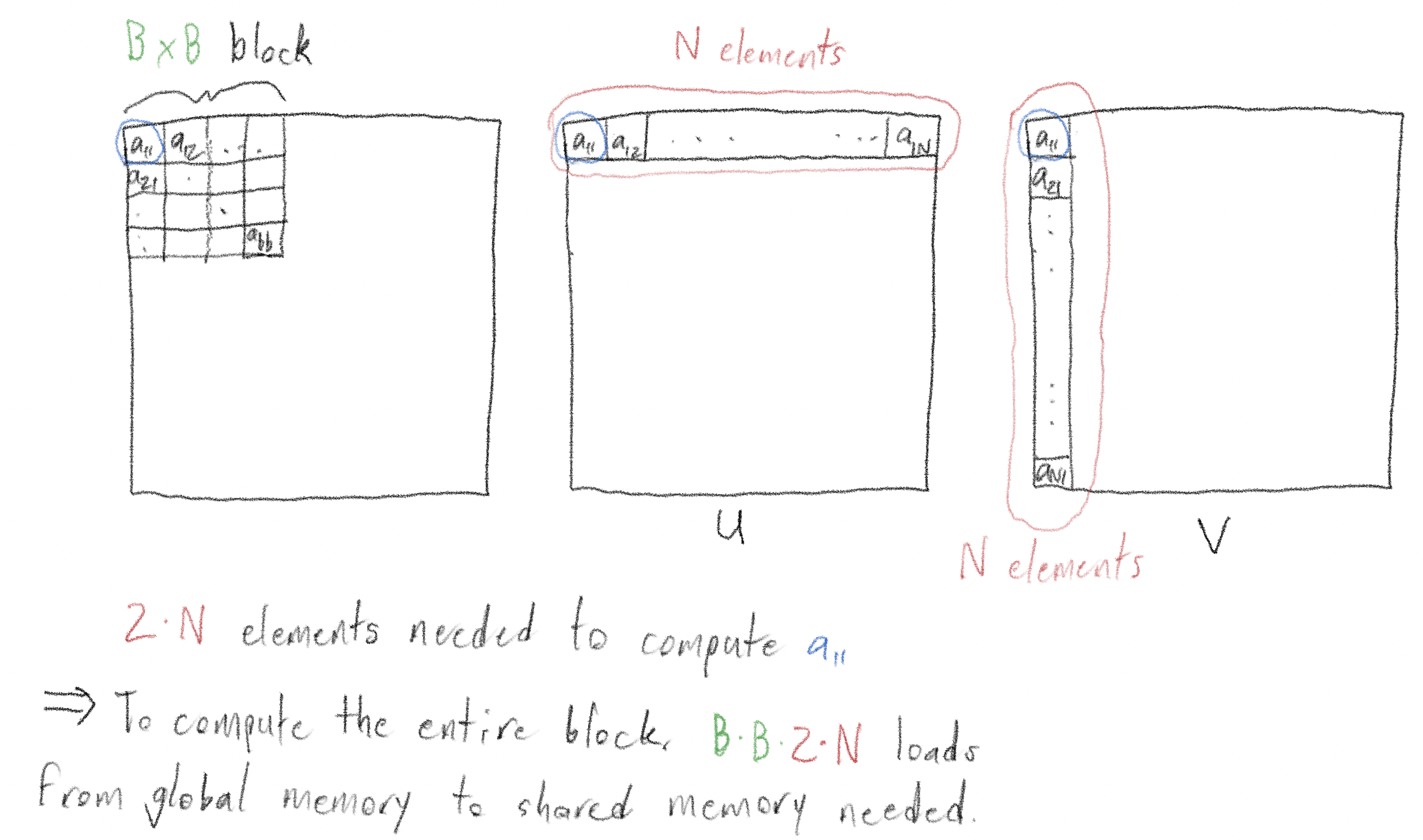
The answer is straightforward: to compute an individual element, you’d need to read in \(2N\) elements, and take the dot product of their vectors. You’d need to do this \(B \times B\) times, once for each of the \(B^2\) elements in the \(B \times B\) block. So there are a total of \(2NB^2\) reads from global memory into shared memory.

Now, we’ll walk through a way of using shared memory to do the same matrix multiplication with \(B \times\) fewer reads from global memory into shared memory! At the end, we’ll show using a simple experiment that this does in fact make the multiplication faster.

Step 1:

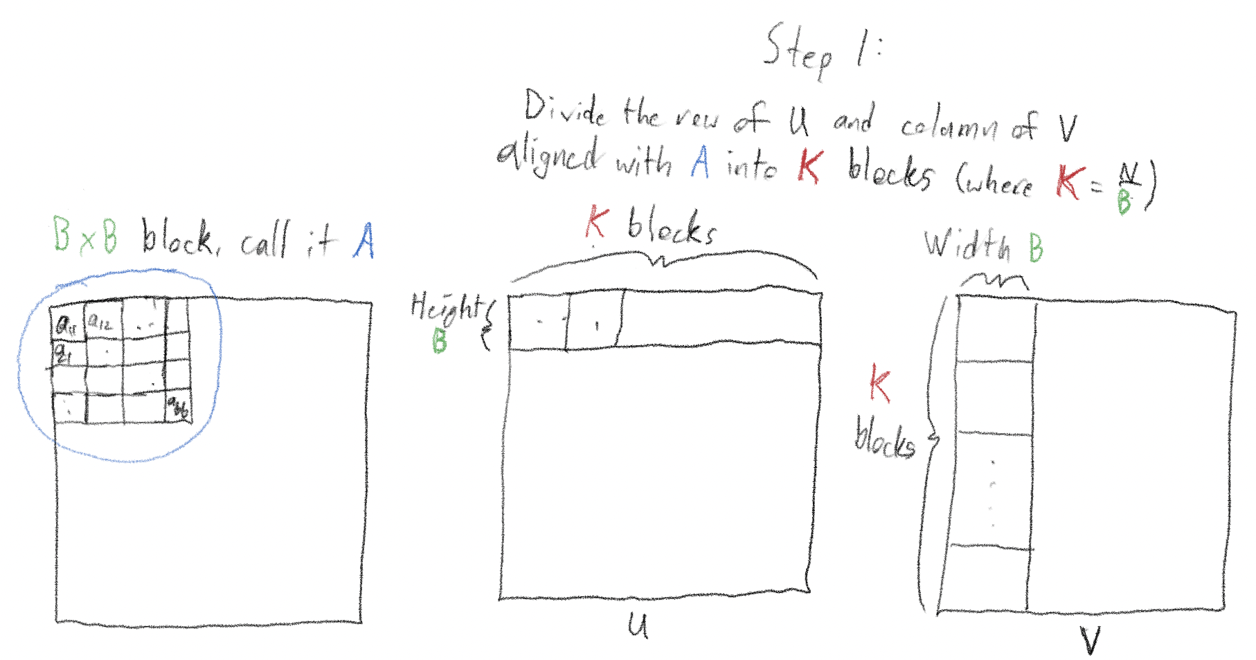
Consider the \(B \times B\) block at the top left of the matrix - call it “A”. Divide the “\(B \times N\)” row containing A into \(K\) blocks (by construction, \(K = \frac{N}{B}\)).

Divide the column containing A, \(N\) rows by \(B\) columns into \(K\) chunks similarly.

Step 2:

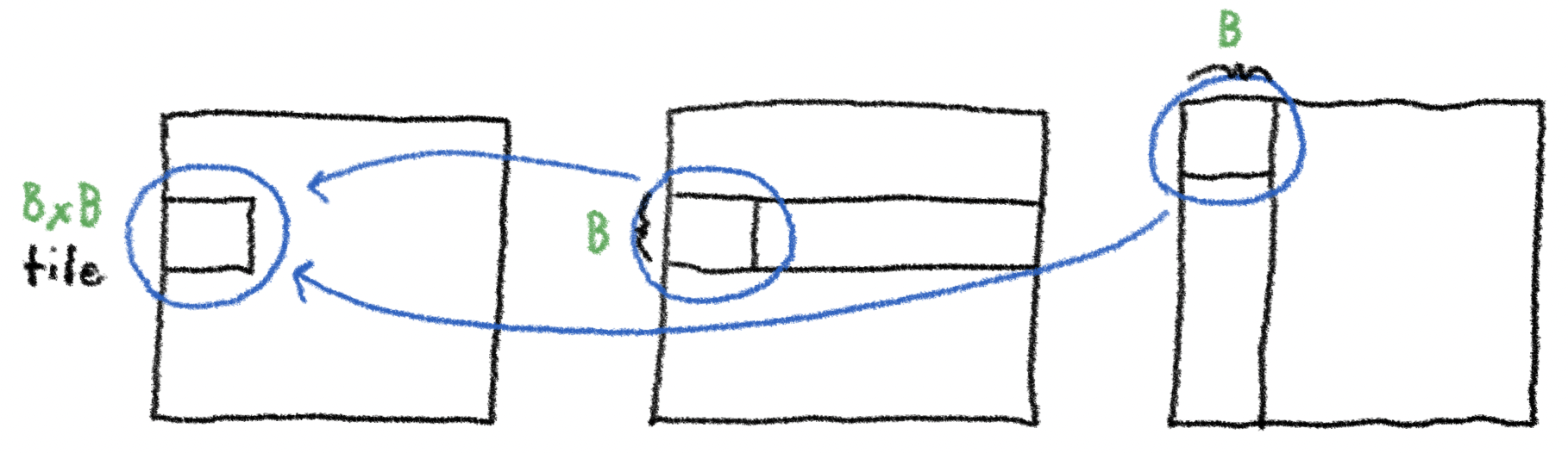
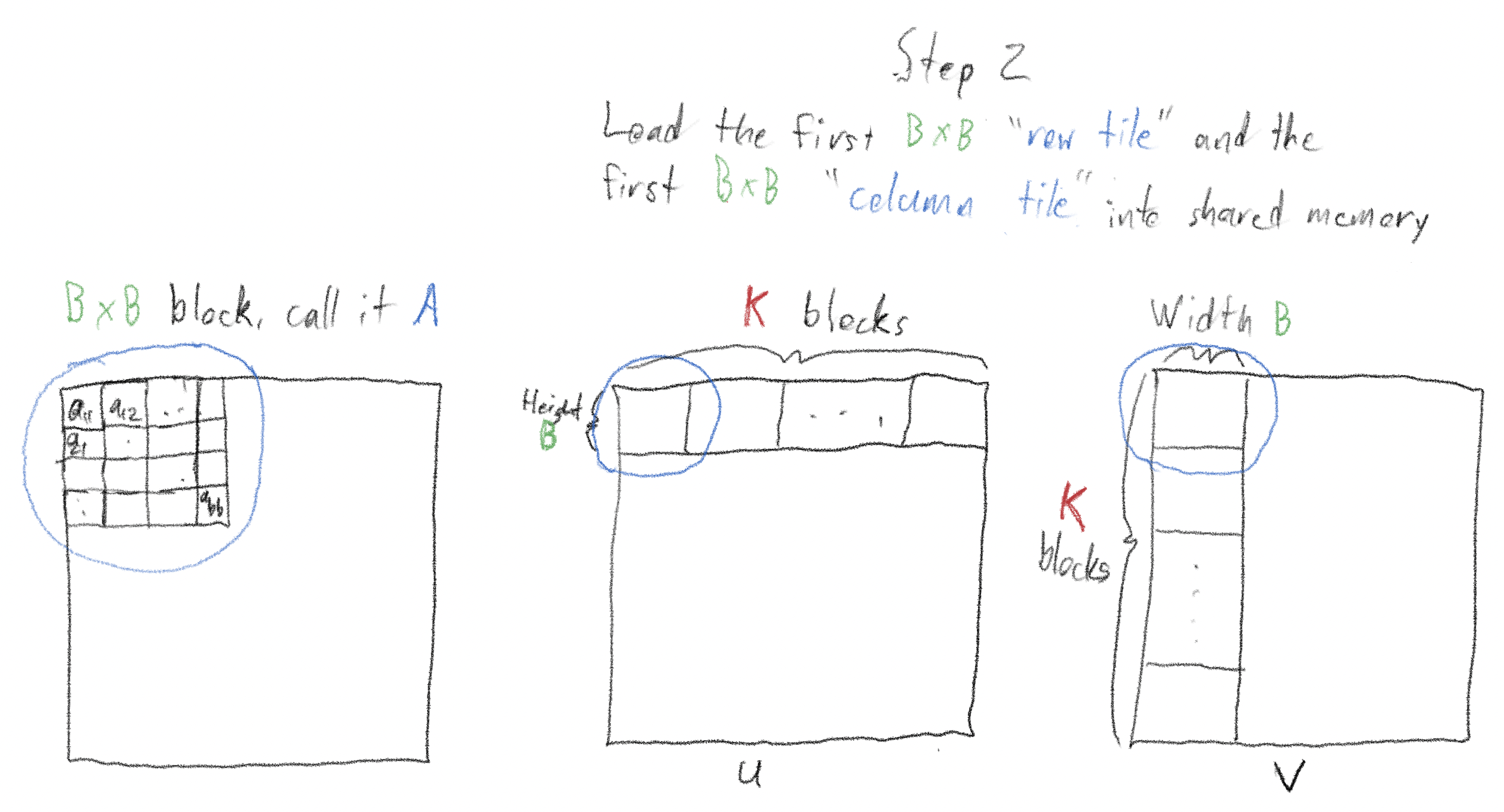
Launch many threads, and use these threads to load the first “tile” - “tile” is the technical name for these “chunks” - of each of the “row slice” and “column slice” into shared memory. Do this in parallel using all the threads; when finished, we will have a \(B \times B\) "row tile" and a \(B \times B\) "column tile" loaded into shared memory. Finally, "sync threads", ensuring that the entire "row tile" and "column tile" are loaded into shared memory before proceeding.

Step 3:

Here’s the clever and beautiful part: use these two tiles to increment, though not fully compute, each of the \(B \times B\) sums in A.

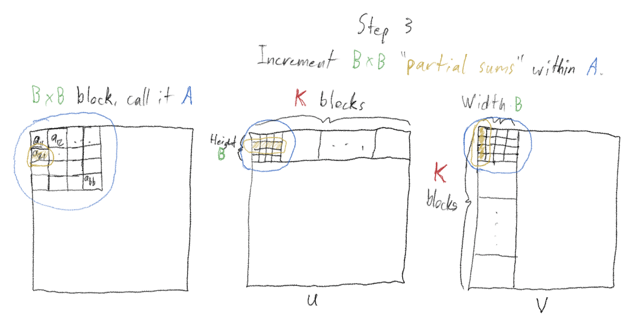
For example, to increment the element in the second row, first column of A, we perform the dot product of the second row of the “row tile” with the first column of the “column tile”, and add it to the ongoing sum of that element.

After this step, "sync threads" a second time, ensuring that all partial sums have been incremented.

Step 4, and beyond

Move on to the next “row tile” in the row containing A and the next “column tile” in the column containing A (if we were incrementing a tile counter \(k\) started at 1, we’d be incrementing it to 2). We’d then perform the same operations as in step 3, incrementing each of the \(B^2\) elements of A.

Step 5

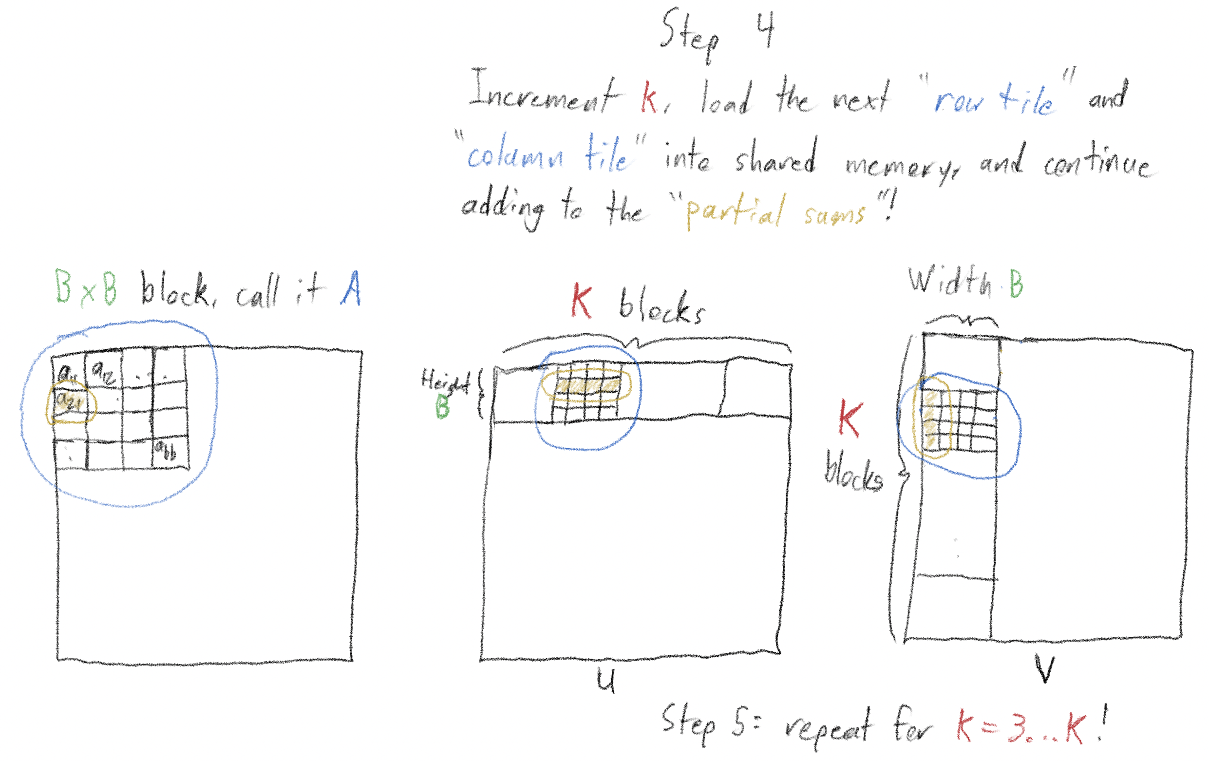
Repeat this process for \(k = 3, 4,\ldots,K\)! By the time we’ve iterated through all \(K\) tiles, we’ve computed the full value of all the elements of A!⁵

Analysis

We read in a total of \(2B^2\) elements on each of \(K = \frac{N}{B}\) iterations, for a total “global -> shared memory cost” of \(\frac{2NB^2}{B} = 2BN\). This is \(B\) times less than doing the reads naively!

Implementation and Benchmarking

I have an implementation here. I would not have been able to write it without referencing:

• This implementation from the GitHub page of Stanford’s CS149 (Parallel Computing) course (my implementation is in my fork of this repo).
• This blog post from Lei Mao (now an engineer at Meta; he was at NVIDIA when he wrote this)

There’s a lot going on in the implementation, but notice that these lines are the ones where two “tiles”, each 2D arrays of size BLOCK_DIM × BLOCK_DIM are initialized, using the __shared__ CUDA C++ keyword. In addition, in line with the explanation above, you'll see two uses of __syncthreads(). Other elements of the implementation, such as the use of threadIdx.x and threadIdx.y to make the implementation more elegant, could be worth another blog post!

Benchmarking against the naive approach

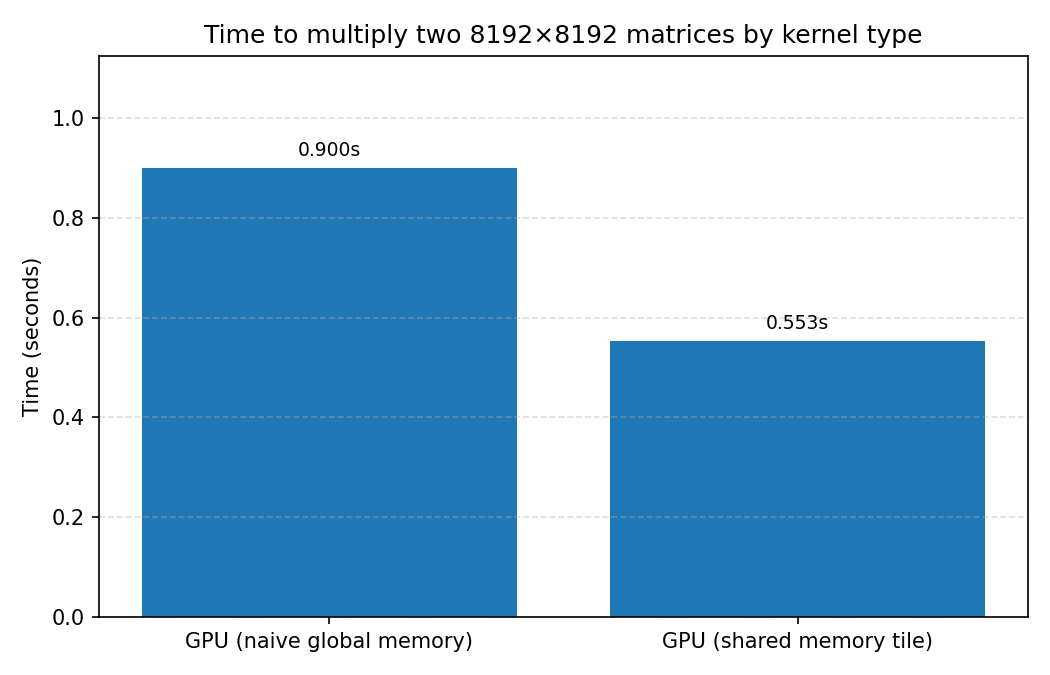
The README shows about a 40% speedup in using the shared memory approach vs. the naive approach (even if the naive approach still uses parallelism) - 553 ms vs. 900 ms!

Benchmarking against PyTorch

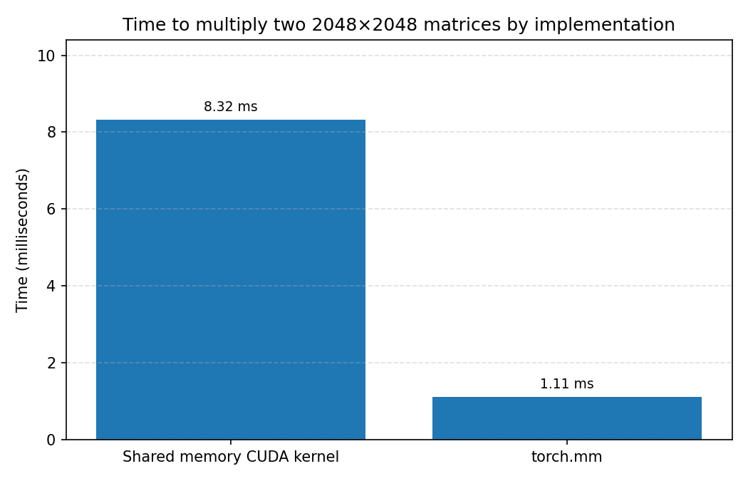
Lest you be impressed: this comparison shows separately that the custom kernel shown here is about \(8 \times\) slower than just calling “torch.mm”! This is because torch.mm uses much-more-highly optimized CUDA kernels under-the-hood.

Conclusion

This blog post covered some basics about CUDA programming, how those basics lead to a common pattern for writing "GPU-aware" code, and how that pattern can be used to speed up matrix multiplication. This pattern is very prevalent throughout AI coding; the widely-used FlashAttention technique uses a similar pattern to speed up the attention computation. Look for a deeper dive on FlashAttention in a future blog post!

Footnotes

¹ There are lower levels of memory beyond the three listed here, but for the purposes of this blog post we focus on these, especially the distinction between global and shared memory. ↩

² Interestingly, CUDA leaves it up to the programmer, if operating on a matrix of total size \(X\), and wanting to use \(N\) threads per block, to compute the number of blocks of threads correctly as roughly \(\lceil X / N \rceil\). ↩

³ To the best of my knowledge, it’s a coincidence that “shared memory” and “Streaming Multiprocessor” both have the initials “SM”. In CUDA-land, “SM” always refers to a “Streaming Multiprocessor”. ↩

⁴ Roughly: a single float32 = 4 bytes. Thus, an 8B parameter model is 32 GB. The L4 GPU I used for these experiments has 24 GB of memory. Quantizing the float32 to float16 cuts the 32 GB down to 16 GB. For inference, this 16 GB would be all that is needed, meaning we could run inference with a 16 GB model on a single L4 GPU with quantization. For fine-tuning, some extra memory would be needed; and for a full training run, 2–4× the memory of this 16 GB would be needed (2x for the gradients alone). ↩

⁵ Astute readers will ask: why not load the entire matrices you're trying to multiply into shared memory? The answer is that there usually simply isn't enough space. Each of the 58 SMs on an L4 GPU supports up to 100 KB of shared memory. This means they could fit two 64 x 64 matrices (4 bytes * 64 * 64 * 2 is about 32 KB), but even two 128 x 128 matrices (about 128 KB) would be too large. As the footnote above mentions, quantization changes this. ↩