A Trick Powering FlashAttention
December 15, 2025
Softmax is an essential operation in AI computing, taking in a vector and returning a normalized vector that sums to one. However, the normalization step means every element depends on all of the other elements in the vector. Nevertheless, in this essay, we'll cover a beautiful trick that lets vector functions closely related to softmax, such as:
be computed in an "online" or "streaming" fashion, meaning that we process the of vectors one chunk at a time without loading the entire thing into memory. As it turns out, streaming the second of these, "softmax dot", is an essential component of the whole family of FlashAttention algorithms (a family of GPU kernels that compute attention using a "tiling" approach similar to the one described here). Instead of diving into "softmax dot", we'll start by showing how the core trick works in the even simpler setting of "the sum of scaled exponentials".
As a refresher, the definition of softmax for a vector \(\mathbf{x}\) is:
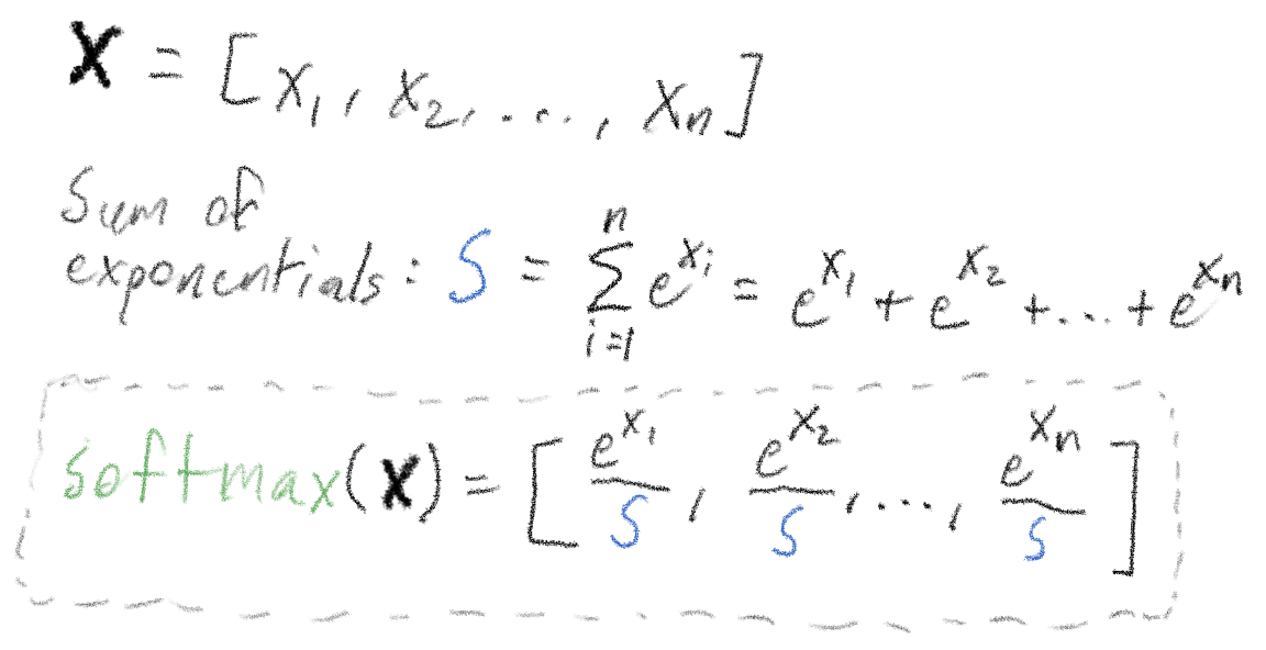
All those exponentials could lead to the values in the softmax vector getting large enough to lead to numeric instability. Softmax has an extremely interesting property that allows us to ensure numerical stability:
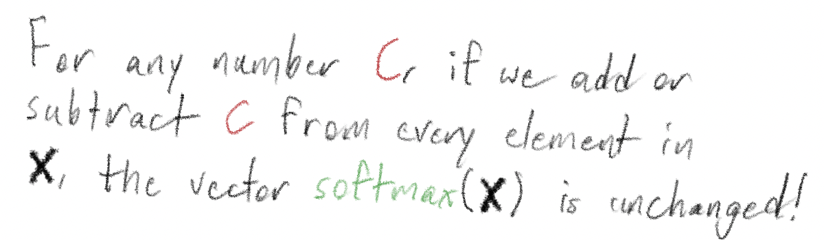
Below is the math that shows why this is the case: for any given index \(j\) (1, 2, and so on up to \(n\)), the "jth element" of the vector \(\operatorname{softmax}(\mathbf{x} - c)\) is:
\[ \frac{e^{x_j - c}}{\sum_{i=1}^n e^{x_i - c}} = \frac{e^{-c} * e^{x_j}}{e^{-c} * \sum_{i=1}^n e^{x_i}} = \frac{e^{x_j}}{\sum_{i=1}^n e^{x_i}} \]Taking advantage of this property, in AI computing, we almost always subtract the maximum value of the vector (\(M = \max(\mathbf{x})\)) from every element prior to the softmax operation. This ensures the largest element of softmax(\(\mathbf{x}\)) is \(e^{m-m} = e^0 = 1\), and avoids us having to compute, for example \(e^{22}\) which is about 3.5 billion or \(e^{222}\) which is almost one googol.
So we want to compute the sum of the exponentials of the vector elements, while subtracting the maximum of the vector and thus ensuring numeric stability; that is, we want to compute:
\[ L = \sum_{i} e^{x_i - M} \]Where \(M\) is the maximum of the entire vector \(\max(\mathbf{x})\).
How can we do this in a “online” fashion? That is, only ever “loading” one chunk of \(\mathbf{x}\) at a time? Clearly, the difficult part is “keeping track of the maximum": theoretically we can't know what \(M\) is until we’ve seen the entire vector, but we still want to process each chunk as it comes in. We’ll now show "proof by induction" style, how to do this.
Suppose we get the first block of, say, 50 elements. We can compute the maximum of this block; let's call it \(m_1\). We'll then "scale the exponentials by \(m_1\)" (we'll re-use this "scale by \(m_1\)" terminology later), meaning we first subtract \(m_1\) from each elements, take the exponentials, and sum the elements. So the sum of this block will just be \[ s_1 = \sum_{i=1}^{50} e^{x_i - m_1} = e^{x_1 - m_1} + e^{x_2 - m_1} + \cdots + e^{x_{50} - m_1}. \]
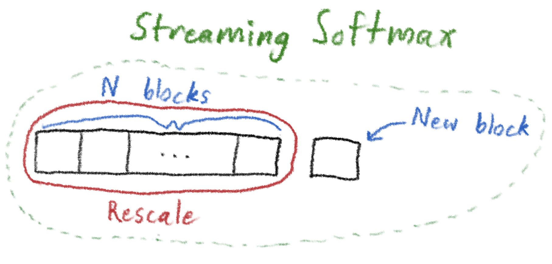
Now suppose we have processed some number of blocks - say nine of them - and we have a running maximum \(M_9\) and a running sum \(S_9\), where the running sum is appropriately scaled by the maximum we have seen so far (clearly, thinking about the prior paragraph, after the first block, the elements will be correctly scaled by the maximum seen so far, \(m_1\)). What do we do upon receiving a new, tenth block of 50 elements?
Let's recall what we have to do: running sum \(S_{10}\), scaled by whatever the maximum \(M_{10}\) is after seeing this block. To update the maximum, we simply take the maximum of what we've seen so far with the maximum of the new block:
\[ M_{10} = \max\left(M_9,\, m_{10}\right). \]How do we update the running sum \(S_{10}\)? There are two cases to consider: the easy case, and the hard case where we'll have to use the elegant "Rescaling Trick" which is the core of this blog post.
First, the easy case: \(m_{10}\) is smaller than \(M_9\). That is:
\[ M_{10} = \max\left(M_9,\, m_{10}\right) = M_9 \]Then if the new block's elements are
\[ b_1, b_2, \ldots, b_{50} \],we can simply add
\[ e^{b_1 - M_9} + e^{b_2 - M_9} + \cdots + e^{b_{50} - M_9} \]to the running sum \(S_9\) to get \(S_{10}\). Once we update the new \(M_{10}\) to simply be \(M_9\), we'll be done processing this block.
Now, the hard case: \(m_{10}\) is larger than \(M_9\) (so that \(M_{10}\), the running maximum after we update this block, is \(m_{10}\), the maxmimum of this block). In this case, we have \(S_{9}\), which has been scaled by a smaller number \(M_9\), and we want to adjust it to have a value as if it were actually scaled by what we now know to be the true "maximum seen so far", \(M_{10}\).
Remember what it means for an element to be "scaled by \(M_9\)": it just means that the element \(x_j\) has been transformed to \(e^{x_j - M_9}\). Look what happens when we multiply such an element by \(e^{M_9 - M_{10}}\):
\[ e^{x_j - M_9} \cdot e^{M_9 - M_{10}} = e^{x_j - M_9 + M_9 - M_{10}} = e^{x_j - M_{10}} \]Thus, multiplying by \(e^{M_9 - M_{10}}\) transforms \(S_{9}\) into what its value would be if it had been scaled by \(M_{10}\) all along. It turns out that indeed, multiplying by \(e^{M_9 - M_{10}}\) "rescales" \(S_{9}\) in exactly the right way. Note why this makes sense intuitively: since \(M_9\) is smaller than \(M_{10}\), \(e^{M_9 - M_{10}}\) is a number between 0 and 1. In some sense, we were "too optimistic" with \(S_{9}\) previously, scaling it according to a maximum that was smaller than the actual maximum by which we should have been scaling it.
These two scripts on GitHub here implement this. The first script shows the rescaling happening concretely when processing a vector in two chunks; the second script shows that the code still works - that is, the sums when processing this vector the normal way and the streaming way are identical - when processing a vector of length 1,000 filled with random integers between 0 and 100, processed in blocks of 50.
The second vector function we cover here is slightly more complicated, and also more directly tied to attention - but it relies on the same straightforward trick in order to stream it!
The second vector-to-scalar function I call \(\operatorname{softmax\text{-}dot}\): the "\(\operatorname{softmax\text{-}dot}\)" of two vectors \(\mathbf{q}\) and \(\mathbf{v}\) is:
\[ \operatorname{softmax\text{-}dot}(\mathbf{q}, \mathbf{v}) = \operatorname{softmax}(\mathbf{q}) \cdot \mathbf{v} \]
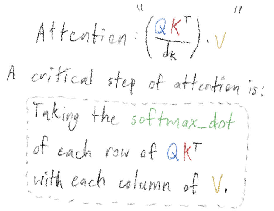
One of the core steps in attention can be described in terms of this operation. Attention is often written in the following technically-correct way that nevertheless barely, if at all, elucidates the ideas involved:
\[ \operatorname{Attention}(Q, K, V) = \operatorname{softmax}\left(\frac{QK^T}{\sqrt{d_k}}\right)V \]I bring this up just to make the following point about where softmax-dot is used in this:
Now that we're motivated, let's actually discuss how to compute this thing.
So how can we actually stream this sum? First, note that each entry of \(\operatorname{softmax}(\mathbf{q})\) is the fraction \(\frac{e^{q_j}}{\sum_{i=1}^n e^{q_i}}\). Therefore, we can rewrite \(\operatorname{softmax\text{-}dot}(\mathbf{q}, \mathbf{v})\) as:
\[ \operatorname{softmax\text{-}dot}(\mathbf{q}, \mathbf{v}) = \frac{\sum_{i=1}^n e^{q_i - M} * v_i}{\sum_{i=1}^n e^{q_i - M}}, \qquad M = \max_j q_j. \]
But we know how to stream both of these! We can calculate the denominator,
\[ e^{q_1 - M} + e^{q_2 - M} + \cdots + e^{q_n - M}. \]
in a streaming fashion using exactly the method we just covered in the prior section - it is literally a sum of scaled exponentials! And the numerator,
\[ e^{q_1 - M} * v_1 + e^{q_2 - M} * v_2 + \cdots + e^{q_n - M} * v_n. \]
can be streamed using the same high level method as the sum of scaled exponentials - keeping track of the maximum of each block, and using the Rescaling Trick on the "accumulated sum" when we get a block with a greater maximum than we've seen so far, etc. - except that we add elements like \(e^{q_i - M} * v_i\) to our running sum instead of elements like \(e^{q_i - M}\) as before.
The key point is that the same rescaling trick works for softmax-dot: the trickiest part of this computation is dealing with the fact that the maximum value of \(\mathbf{q}\) we've seen so far can change as we get more elements, and we handle both checking for that and rescaling using \(e^{m_{old} - m_{new}}\) in exactly the same way!
As with the first two scripts, the third script in the GitHub repo shows that for two length 100 vectors of random floats between 0 and 2 (arbitrarily), computing the softmax-dot the normal way and the streaming way yields the same result.
The block-by-block computation of the softmax-dot operation, along with the tiling approach discussed in my previous post is the secret sauce behind the massive speedups seen in FlashAttention. In a future post and/or implementation, we'll put these ideas together to show how a fuller version of FlashAttenion works.