How Tiling and Streaming Softmax Enable this GPU Kernel
January 27, 2026
This blog post will explain the FlashAttention algorithm, showing how it builds upon the concepts from two prior blog posts: tiling, and streaming softmax. More specifically, this post will focus on a "whiteboard-level" understanding of the algorithm, and, where helpful, will link out to a Python implementation that mimics how the algorithm would be coded in CUDA; we'll save a full CUDA walkthrough for a future blog post (though readers may find it a good exercise to implement FlashAttention in CUDA after reading this blog post, using the Python implementation as a starting point).
FlashAttention is a drop-in replacement for many of the steps of the Multi-Head Attention operation, which itself is the foundational building block for modeling sequences introduced in Attention is All You Need and is described in more detail (with a couple reference implementations) in a prior blog post here. It was released in mid-2022 by a team led by Tri Dao, then at Stanford. This release, now known as "FlashAttention V1", already provided a13% speedup over highly-optimized CUDA kernels written by NVIDIA for their own GPUs! These impressive speedups were achieved because FA V1 was the first to apply the concepts covered in this series of posts - tiling and streaming softmax - to the core Multi-Head Attention operation. Subsequent versions have employed much more sophisticated software features of GPUs, some of which only work on the most recent NVIDIA GPU generations, and have had varying degrees of involvement from Prof. Dao1, but the basic ideas introduced in V1 continue to be core and are what produced the original "great leap forward" in Multi-Head Attention performance on GPUs.
FlashAttention is sometimes described as "a drop-in replacement for attention". That is not entirely accurate; it replaces many of the steps involved in Multi-Head Attention, but not all. Below is a reminder of all the steps involved in Multi-Head Attention:
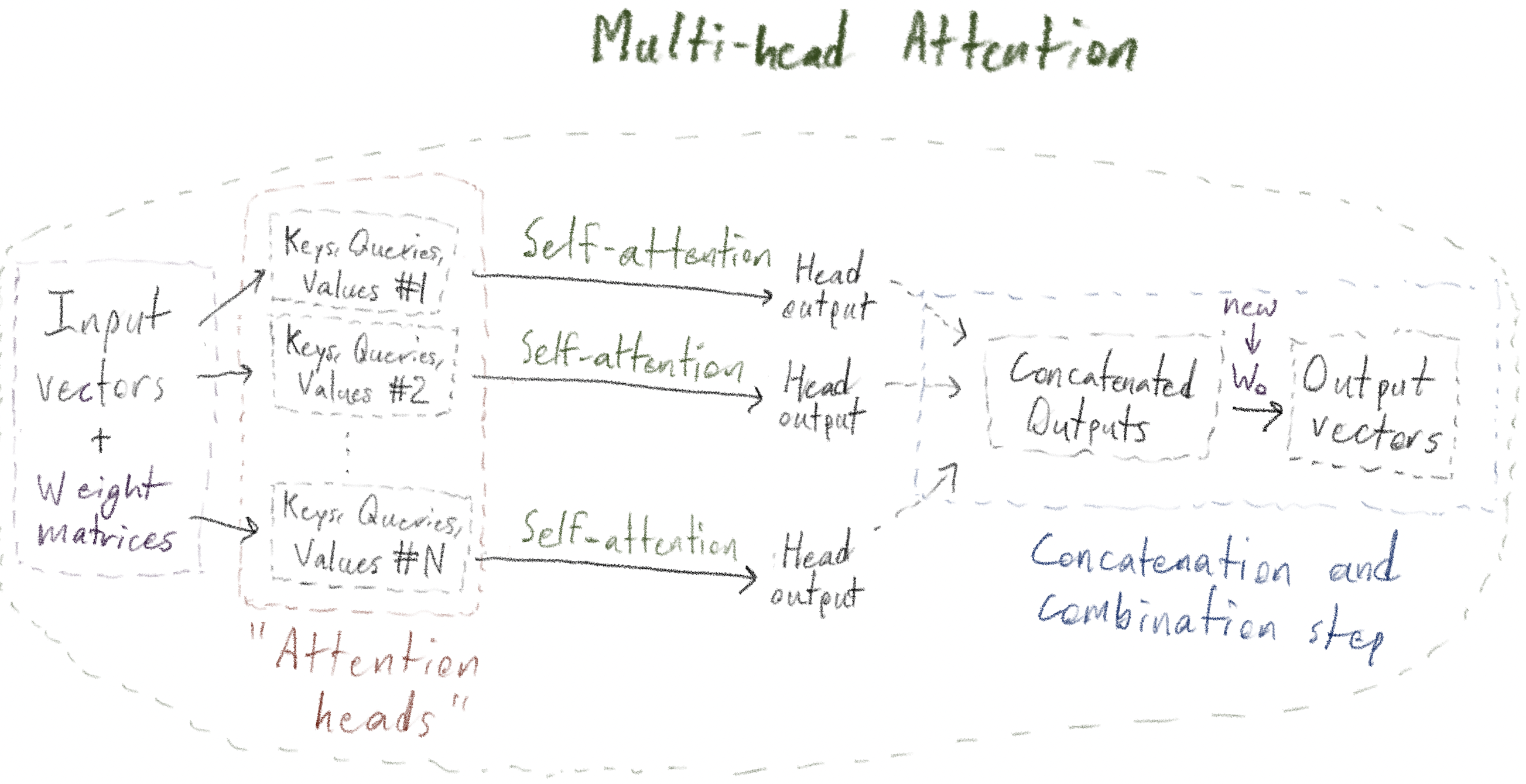
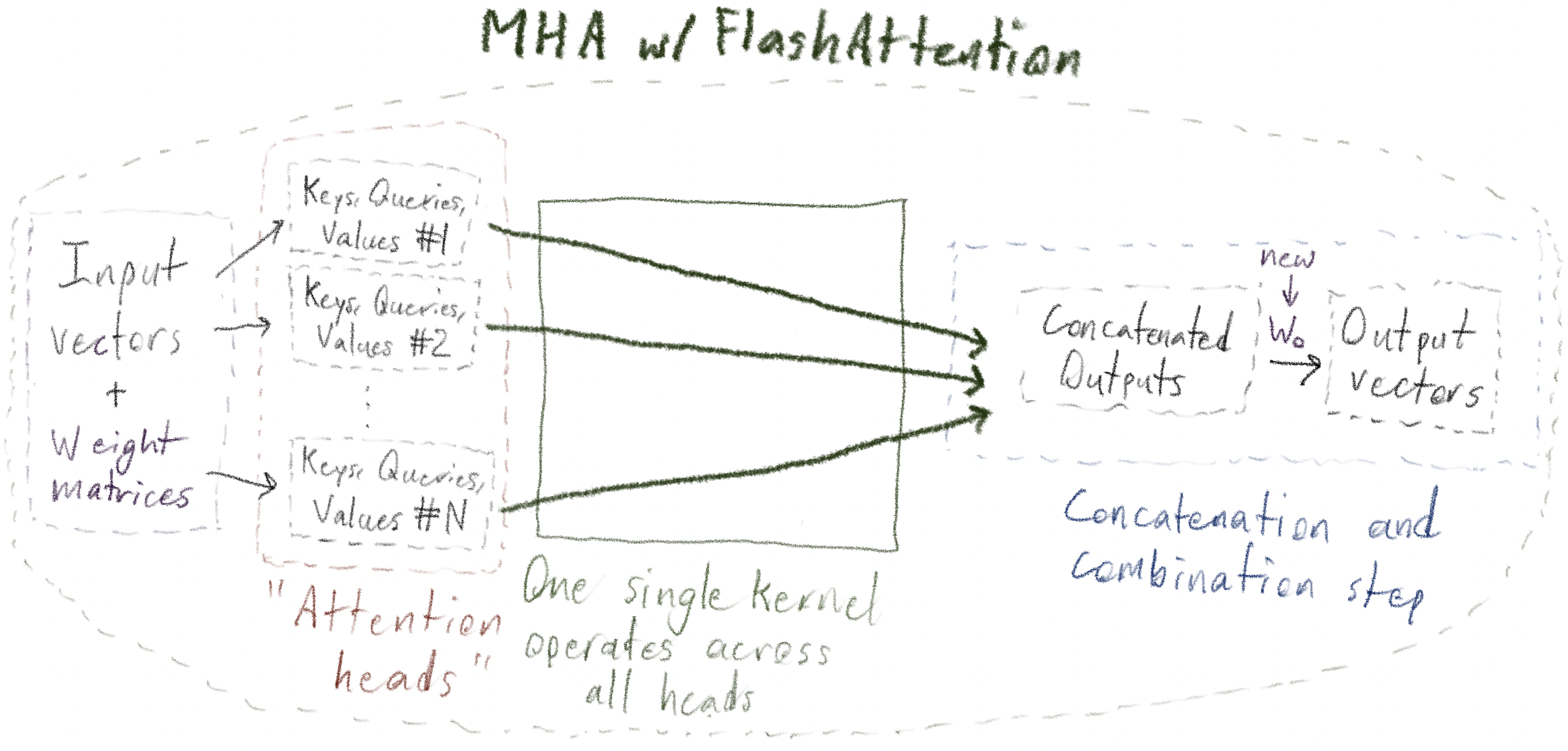
FlashAttention fuses a particular key sequence of these operations into a single CUDA
kernel; in particular, standard Multi-Head Attention requires "materializing" -
defining and holding as one object in memory - entire "sequence_length
× sequence_length" attention matrices within each head, whereas
FlashAttention is able to compute the same final result while avoiding this
memory-intensive materialization.
Note that, for example, the final step of multiplying the concatenated outputs \(W_O\) is not part of the FlashAttention kernel.
So how does it do it?
We'll start with three high level comments on FlashAttention that can keep you oriented when going through the specific steps of the algorithm:
In this blog post, we describe a technique for computing the output of an operation involving two input matrices by:
The structure of what we do in FlashAttention is very similar (which is why reading through and making sure you understand that blog post is great scaffolding for understanding FlashAttention), except now we have three input matrices - \(Q\), \(K\), and \(V\) - and the operation we're trying to "emulate in a tiled fashion" is the attention operation:
\[ \operatorname{Attention}(Q, K, V) = \operatorname{softmax}\!\left(\frac{QK^T}{\sqrt{d}}\right)V \]rather than simply a matrix multiplication.
That raises a question: where do these "two dimensional Tensors" we deal with in
FlashAttention come from? \(Q\), \(K\), and \(V\), after all, are typically
four-dimensional Tensors of shape
[batch_size, sequence_length, head_dim, num_heads] in attention
implementations; even if you discount the batch dimension--operations are always the
same within each batch element in neural networks, so that they are actually
"batch_size" identical operations happening in parallel--you are still
left with three dimensional Tensors of shape:
[sequence_length, head_dim, num_heads]. Here we take advantage of a
further parallel structure in Multi-Head Attention: the computations
within each head are identical. Naturally, then, in FlashAttention v1, we
launch a GPU kernel with a grid of "batch_size * num_heads"
thread blocks, each of which operates on a single
(batch_index, head_index) tuple. Each thread block will then operate on
the three "sequence_length × head_dim" Tensors:
Q[batch_index, head_index, :, :]
K[batch_index, head_index, :, :]
V[batch_index, head_index, :, :]
and produce the "sequence_length × head_dim" Tensor
O[batch_index, head_index, :, :]. So, the algorithm we'll describe
starting in the next section really is a "three 2D matrix" analogue of the "two 2D
matrix" tiling algorithm described in the
prior blog post; "the magic of CUDA" (specifically
being able to launch "batch_size * num_heads" blocks of
threads at once) scales this up to be the 4D Tensor operation we need.
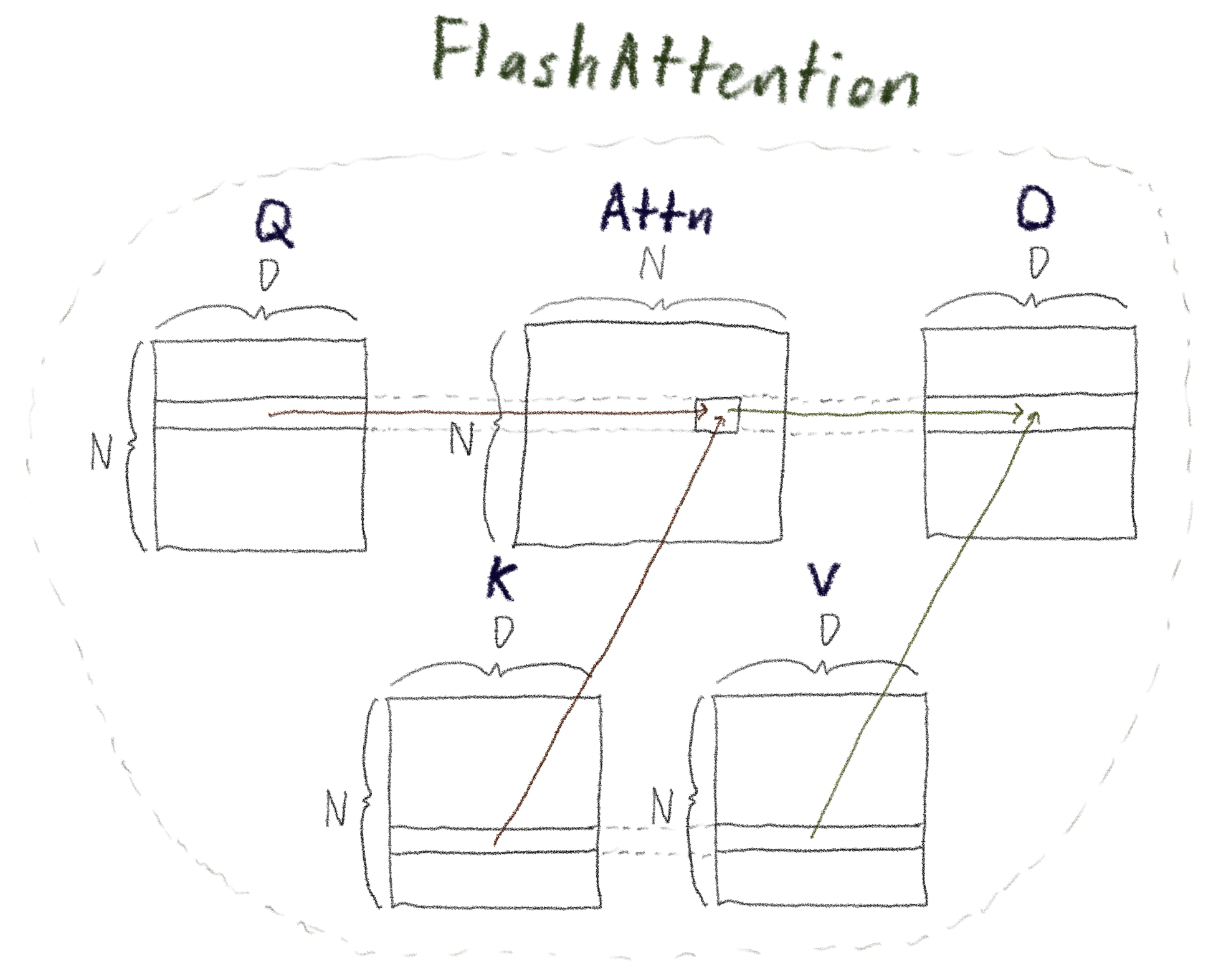
Now that we understand that we can operate on two dimensional slices of \(Q\), \(K\), and, \(V\), we have to get to the core of the problem: how we are going to "tile" these to compute \(O\) without ever computing the full attention matrix.
If you dive into a single row of the output matrix \(O\), you'll see that it only depends on the values from the corresponding row in \(Q\)! Incidentally, it turns out each element of this row will actually depend on all elements of \(K\) (due to the softmax operation), and all of the elements in the same column as that element within \(V\). Independently of this latter detail about \(K\) and \(V\), the point is that collectively the row needs to "see" all rows of \(K\) and \(V\) whereas it only needs to see the corresponding row of \(Q\). This leads to the tiling strategy described in the next section.
In the diagram and the text below, we'll use
- \(N\) to refer to the
sequence_length- \(D\) to refer to the
head_dimMoreover, we refer to a Python re-write of the CUDA kernel that may be easier for readers to grok and/or hack on themselves than the CUDA C++ code.
As with the blog post where we covered matrix multiplication, the picture showing the geometry of what is going on is critical. The key picture is below:
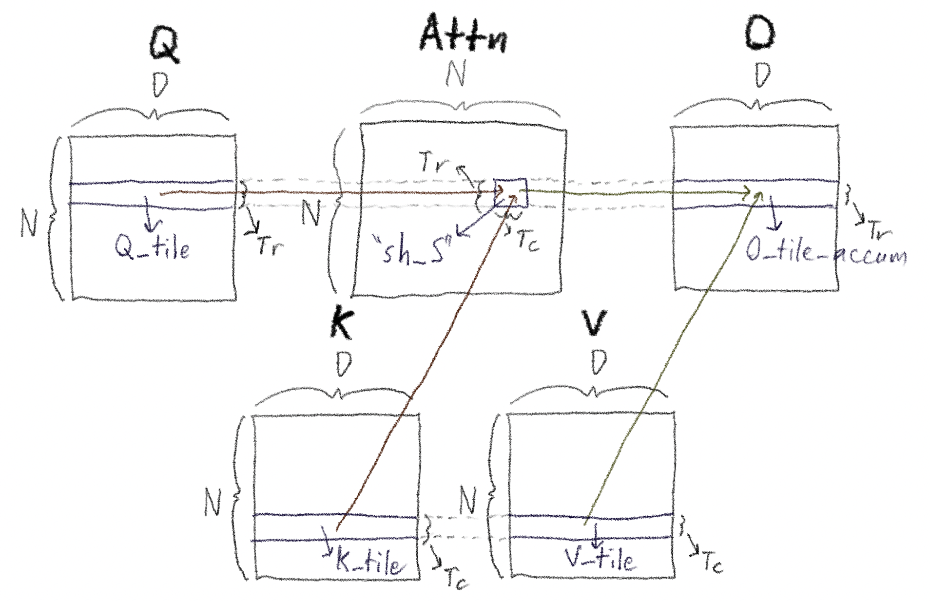
Outer loop (over query tiles): We load in a tile of \(Tr\) rows of \(Q\) — call it \(Q_{tile}\).
Inner loop (stream over key/value tiles while \(Q_{tile}\) is loaded into shared memory):
While this is loaded in, we
loop through
\(K\) and \(V\), \(Tc\) rows at a time (the c is for columns;
you’ll see why shortly).
For each \(K_{tile}\),
we take the dot product of \(Q_{tile}\) with \(K_{tile}^T\); this creates a "\(Tr\) rows by \(Tc\) columns" matrix of sums that, in the
\(N \times N\) attention matrix, sits in the same set of rows as
\(Q_{tile}\) and the same set of columns as \(K_{tile}\). We call this
sh_S--sums stored in shared
memory--in the code. We
record the maximum value
seen for each row in this block.
We "rescale these sums", motivated by the ideas from the streaming softmax blog post. Remember that since softmax is itself a fraction, the attention operation (ignoring the scaling factor) can be written:
We know how to compute this in a "streaming" fashion: we update the running
max, and use this updated max to compute the "scaled exponentials"
themselves as well as adding to the running sum and rescaling it if necessary.
These two operations happen
here
and
here
respectively. For an individual row_in_q_tile row, we store the
running denominator in row_sumexp[row_in_q_tile] and the running
max in row_max[row_in_q_tile] to be used later.
We
multiply
these now-scaled rows by the corresponding \(V_{tile}\) to get a "Tr
× D" tile contribution in the same location as \(O_{tile}\).
In code we call this O_tile_accum.
As in tiled matrix multiplication, we
increment
these "Tr × D" elements of \(O_{tile}\), then
move on to the next \(K\) and \(V\) tiles.
After looping through all tiles in \(K\) and \(V\), we’ve accumulated the numerator of softmax-dot for each row.
So the final step is to
divide each row of the accumulated numerator by its stored denominator, which we've stored as row_sumexp[row_in_q_tile].
Back to the outer loop: Move on to the next \(Q_{tile}\) and repeat until all rows of \(O\) are filled.
As should be clear from the diagrams and description of the algorithm above: FlashAttention actually consumes constant memory in the forward pass, whereas a naive Multi-Head Attention implementation would require \(O(N^2)\) memory! Though we won't go into the backward pass in detail in this blog post, it turns out the standard way of computing it, that offers a very good tradeoff between computation and memory, involves saving the per-row maxima and sums of scaled exponentials; this takes up \(O(N)\) memory. Still a huge improvement over \(O(N^2)\)!
Moreover, since this is the section on compute complexity: astute readers will notice that we're clearly "leaving some parallelism on the table": since each \(Q_{tile}\) is independent, we could clearly parallelize so that we running through the algorithm above on multiple \(Q_{tile}\)s at once! This is done in FlashAttention V2; this quote from the abstract, listing the key improvements in FA V2:
...(2) parallelize the attention computation, even for a single head, across different thread blocks to increase occupancy...
describes exactly this.
This post covered how tiling and streaming softmax enable us to compute large parts of the Multi-Head Attention operation without ever materializing the entire attention matrix, along with pseudocode that should make the algorithm more concrete. In a future blog post we'll walk through the CUDA side of the implementation in more detail; for now, this should provide a clean implementation you can look through.
1 FlashAttention v3 Colfax Research--especially Jay Shah--and NVIDIA, whereas FlashAttention v4 (which has only been semi-published, with Tri Dao giving a talk on an early version of it in August 2025) appears to be nearly 2,000 lines of Python CuTe DSL code written by Prof. Dao himself. ↩